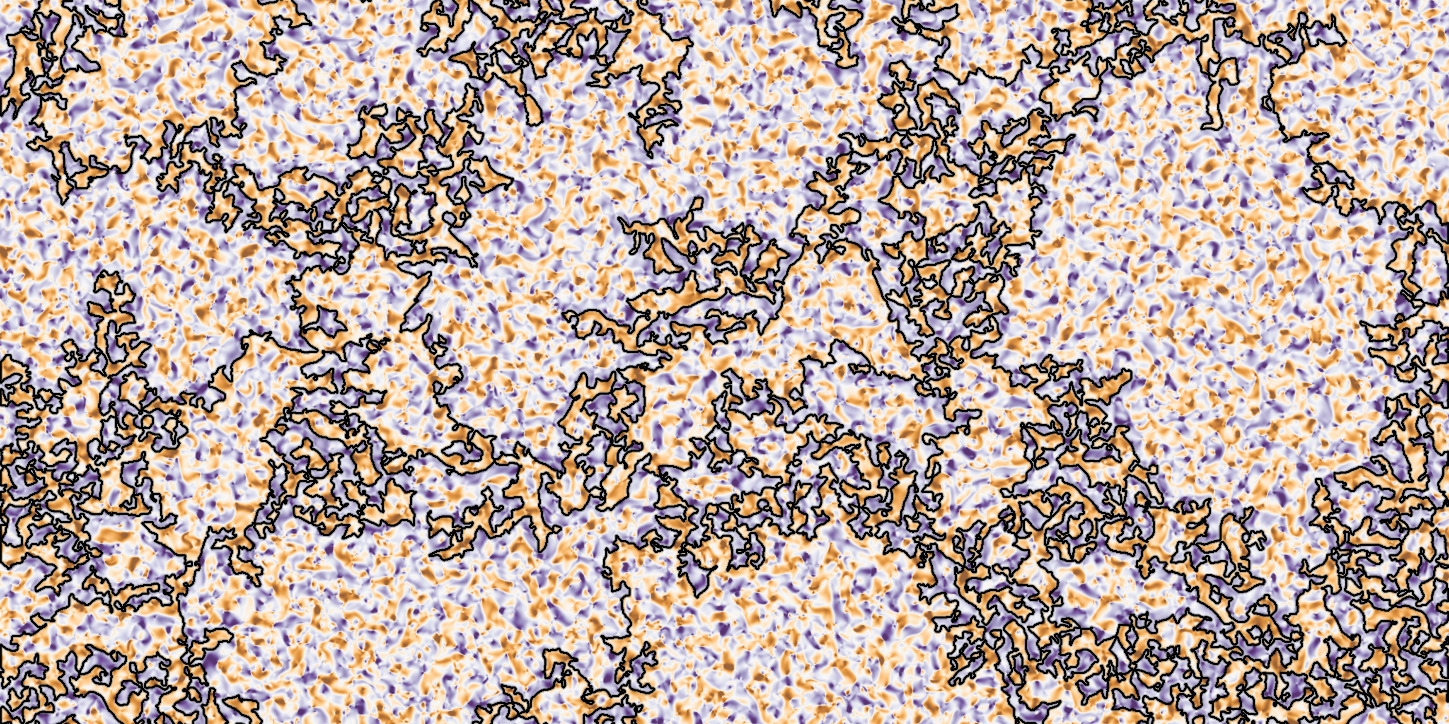
Usually turbulence is driven by an external force; milk being poured into coffee, a waterfall dropping water into a pool, swirls of air when a train goes by. But turbulent-like behaviour can also appear in systems where the fluid stirs itself, where living constituents act to produce complex flows. For example, a dense suspension of swimming bacteria will organise into a flowing state of many vortices, forming and breaking over and over again. A solution of microtubules with their kinesin motors will do much the same.

This behaviour is called active turbulence, due to the striking visual similarity to turbulence observed in more everyday fluids, such as milky coffee. However, there is no agreed upon definition of when active systems really reach this turbulent state we call fully developed active turbulence. We set out to find a measure for fully developed active turbulence and found that this state is encoded in the geometry of the flow.

Flow lines point to a universality class

In order to access the geometry, we draw a line between clockwise and anticlockwise rotational flows, the zero-vorticity isoline. This curve is craggy, multiscale, and crosses the whole field. Previous work on this isoline has been able to place this state in the universality class of critical percolation in inertial turbulence and active turbulence [Bernard 2006, Andersen 2025]. This means that the active turbulent state is conformally invariant, encompassing invariance to translations, rotations, rescaling, and angle-preserving transformations.

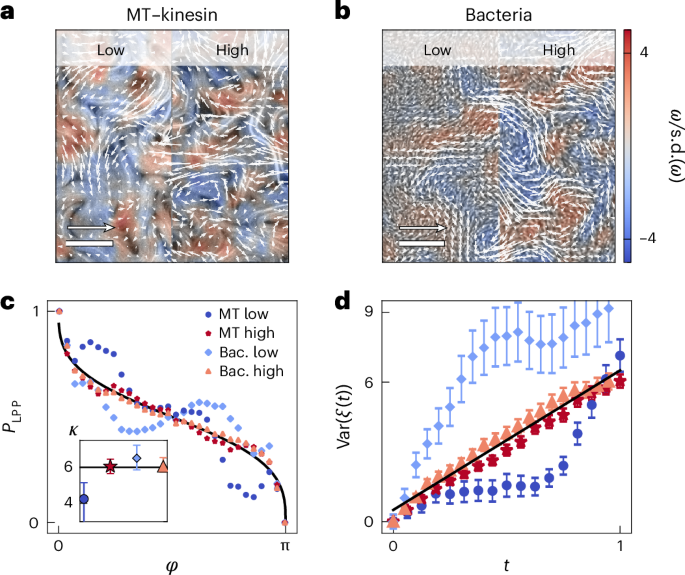
This measurement is made possible by Schramm-Loewner evolution [see Cardy, 2005], a mathematical framework that defines a family of curves controlled by the parameter κ. Different values of kappa (stylised as SLEκ) correspond to different universality classes, and so by measuring in our system, we can place it in a universality class. The aforementioned critical percolation corresponds to κ=6, that is SLE₆. 

The central question is then whether we can use this single parameter to define the state of active turbulence, which exists for a broad parameter range.

A unified descriptor of turbulence across living systems and active models

We set out to test the conformal invariance experimentally using two distinct active systems.

The microtubule kinesin (MT-kinesin) system consists of the rod-like microtubules and the kinesin motors modified such that they can push two microtubules in opposite directions to each other. The mixture is concentrated at an oil-water interface in order to observe two dimensional active turbulence.  We also used Bacillus subtilis bacteria which are self-propelled rod-like bacteria, and at high densities form an active fluid.

An innovative approach, where the ATP that fuels the kinesin motors is released by light, allowed us to study the change in flow behaviour as the MT-kinesin system becomes more active in the same sample. We found that as the activity increased, we could see a transition to SLE6 by measuring the zero-vorticity isoline. We had therefore observed a transition in the flow to the conformally invariant state we call fully developed active turbulence. 

In the case of the bacterial fluid, by sealing the chamber they are in, we can see the activity drop as the oxygen level drops and the bacteria run out of energy. In this case we saw the SLE6 state break as the oxygen ran out.

These experiments were supplemented by simulations of active nematics, a fluid of rod-like particles which exert a non-equilibrium stress on their neighbours. These simulations let us show the transition more clearly. In order to rule out that this was specific to active nematics, we also simulated non-equilibrium fluctuating nematics, in which a mismatch of thermal baths leads to generic non-equilibrium fluctuations, and found the same symmetry-breaking transition.

We had gathered evidence for the transition in two very different experimental systems and in typical active nematics simulations as well as for a more generic non-equilibrium fluctuating nematics model. However, we were not even able to distinguish the states by eye, and we wanted to move to understanding this transition from a physical point of view.

Vortex organisation holds the answer 

We changed perspectives, moving from the single system size zero-vorticity isoline to observing the vortices, which are the centres of rotational flow,  that make up this flow as a point cloud. Understanding this network of vortices proved key to understanding the transition in the flow.

We connected the vortices if the distance between them was smaller than some length r. Clearly, as we increased r we would then go from a totally disconnected to a totally connected network. The way in which the connectivity increased was however totally different. For low activities, the path to connectivity was very slow, with full connectivity not guaranteed until r was many times the average inter-vortex distance l. On the other hand, for fully developed active turbulence, the network became connected at exactly l, with one giant cluster spanning the system and containing most of the vortices.

Going one step further, we investigated the structure of this network. Connecting vortices by rigid edges, we found that the transition to fully developed active turbulence coincided with a rigid network. So at high activity, the vortices are not only well connected but also mechanically constrained by the network they are part of.

Finally, we used persistent homology, a multiscale method to investigate the vorticity fields. Flooding the fields gradually, we counted the number of disconnected islands and lakes in those islands. We performed a principal component analysis on this data and found that the system moves along principal component 2 in the low activity phase, at the transition changes direction and moves along principal component 1 in the fully developed active turbulence phase.

Defining fully developed active turbulence

We can now say that an active fluid reaches fully developed active turbulence when its isolines correspond to SLE₆, that is to critical percolation.

We have therefore developed a measure to pinpoint the transition to fully developed active turbulence which is not dependent on the specific type of activity or system and is proven effective for experimental systems. It is also easy to use and requires only images of the system in question, with no intervention.

Furthermore, we were able to show that in our systems, the transition to SLE₆ coincides with a rigidity percolation of the flow vortices, hinting at an explanation for the conformal invariance.

Plenty of questions are still open. Why do geometric percolation and mechanical rigidity switch on at the same activity, when in equilibrium they belong to different universality classes? Will other living matter, such as cell layers, and other active models show the same transition? Can conformal symmetry become part of a broader theory of systems driven far from equilibrium?

What we have learned is that there is a universal signature of fully developed active turbulence, and that it comes with a structured flow, observable in the vortex centres.

[Bernard 2006] Bernard, Denis, et al. "Conformal invariance in two-dimensional turbulence." Nature Physics 2.2 (2006): 124-128.

[Andersen 2025] Andersen, Benjamin H., et al. "Evidence of universal conformal invariance in living biological matter." Nature physics 21.4 (2025): 618-623.

[Cardy 2005] Cardy, John. "SLE for theoretical physicists." Annals of Physics 318.1 (2005): 81-118.