X-ray computed tomography is a versatile technique for 3D structure characterization, and the pursuit of a faster yet reliable scan is never ended. A lot of methods, such as the maximum likelihood expectation maximization (MLEM) and maximum-a-posteriori (MAP), have been proposed and developed to improve the speed, but most of they are mainly for the "step-scan" mode. At synchrotron facilities such as the FXI beamline at Brookhaven National Laboratory, data is normally collected in the high-speed "fly-scan" mode, which inevitably results in a blurred image using traditional reconstruction algorithms. Figure 1 illustrates how a "fly-scan" mode can introduce artifacts due to the nature of rotation. MLEM and MAP+TV methods can be employed on top of the FBP reconstruction algorithm, however, their performance is still limited (see Figure 3).

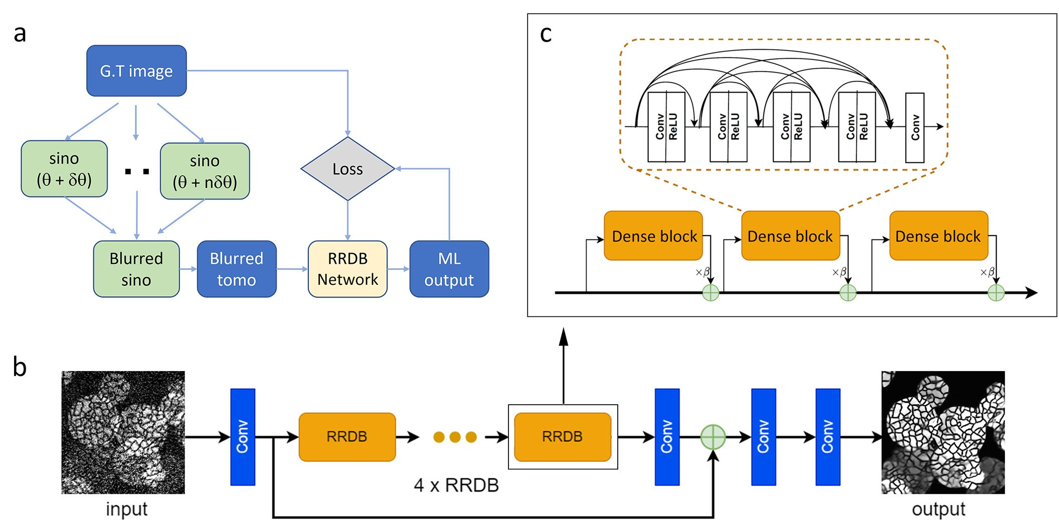
In this work, we are trying to push the fly-scan imaging speed limit further, down to sub-10 second, by using the machine learning (ML) method. We chose the filtered-back-projection (FBP) method that reconstructs the sinogram to get a “blurred tomogram”, acknowledging that the obtained tomogram consists of both blurring artifacts and noise artifacts. The blurred tomogram is then fed into our neural network model, which is composed of three residual-in-residual dense block (RRDB) modules as the backbone and other layers (see Fig. 2b). The RRDB follows the same architecture as stated in the literature, and three modules achieves a good balance between the numerical accuracy and computation speed. The pixel-wise difference between the ML outputs and ground truth is back propagated to update the ML model. We have prepared four types of images with different geometries, feature sizes, and feature types as a general representation of a vast variety of samples that we commonly encountered in the experiments.

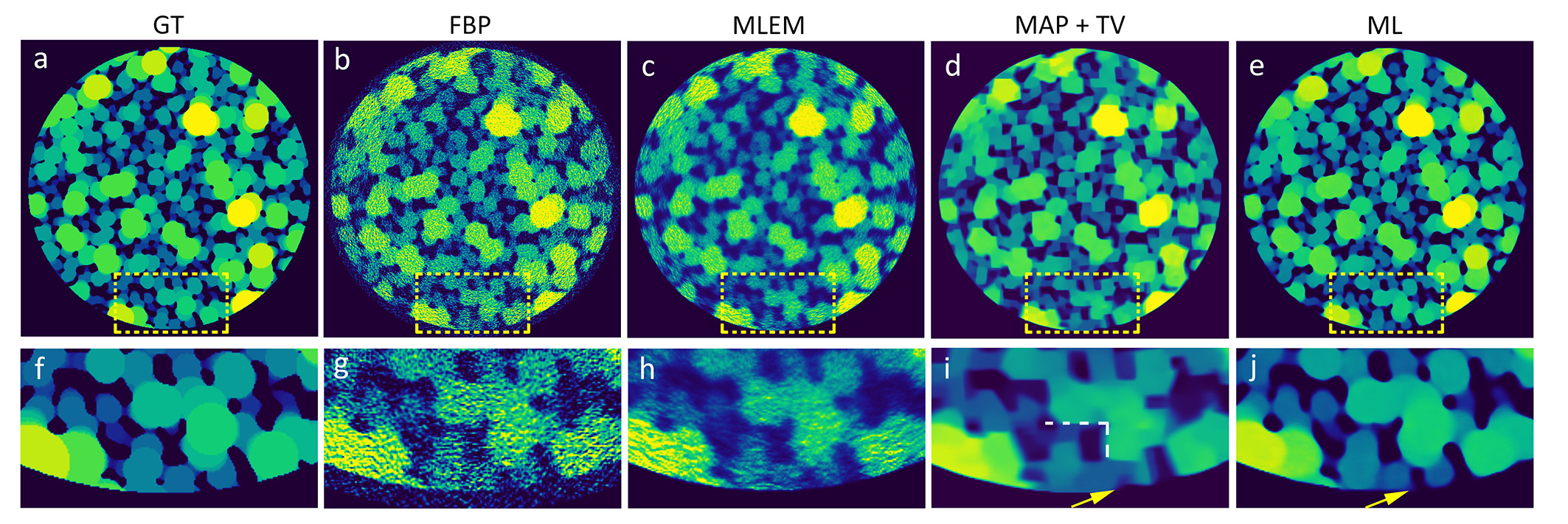
We compare the reconstruction results using different reconstruction algorithms: FBP, MLEM, MAP+TV, and ML. From figure 3, the construction using FBP gives a noisy reconstruction, originating from the limited projections number and the Poisson noise in the sinogram. Reconstruction from MLEM displays strong blurring and noise at the image edge. The noise level in MAP+TV method is largely suppressed, and boundaries are sharply preserved compared to the reconstruction from FBP and MLEM. However, we also note that MAP+TV generates additional artifacts. The reconstruction tends to form straight edges at particle boundaries; the round shape ball-like particles turn into facet ones. The ML results give the closest-to-grand-truth reconstruction. Compared to MAP+TV, ML does not have straight-boundary artifacts and preserves even sharper boundaries for small features than MAP+TV (see the arrows in Figure 3i and 3j). The improved reconstruction quality is also measured by the increased PSNR and SSIM (refer to Table 1 in the original article).

Even though the speedup is not in the magnitude of order's level (currently a typical fly-scan cost is around 1 min), considering the fact that FXI and other similar TXM facilities are supporting worldwide researchers, an even small improvement can save a huge amount of total experiment time!
If you are interested, check out our paper for more details and discuss it here!
Follow the Topic
-
Communications Materials

A selective open access journal from Nature Portfolio publishing high-quality research, reviews and commentary in all areas of materials science.
Related Collections
With Collections, you can get published faster and increase your visibility.
Advanced characterizations of high-entropy materials
Publishing Model: Open Access
Deadline: Mar 31, 2026
Fundamental science and applications of silk proteins
Publishing Model: Open Access
Deadline: Mar 31, 2026


Please sign in or register for FREE
If you are a registered user on Research Communities by Springer Nature, please sign in