
What makes a model useful? The most basic criterion would be to provide meaning. Going further, a good model draws meaning from relevant information and leaves out noise. How then do we know if the patterns picked up by models are meaningful? How much information is required to pick up all of the signals available in any particular dataset? What if there are multiple paths leading to the same conclusions?
In so many microbial ecology papers, authors fit their models on the entirety of their data and proceed to draw conclusions. This is a flawed practice as the conclusions drawn can only reasonably be held true on the stretch of data the models were fitted to, i.e. there is no testing of the models to confirm they are generalizable to similar additional data.
In the context of our paper, we aim at using the smallest possible number of bacterial taxa yielding an accurate classification of river ecological status at sampling sites. We could not just fit our models on all the data and point to the bacterial taxa showing the strongest correlations with ecological status; we had to prove the identified correlations hold true for data points not used for training the model. We also raised the challenge one step further: make accurate predictions of what happens at sites downstream of the input data used to make predictions. In essence, we require of our models that they pick up on community assembly processes over time and space in order to accurately predict future outcomes.
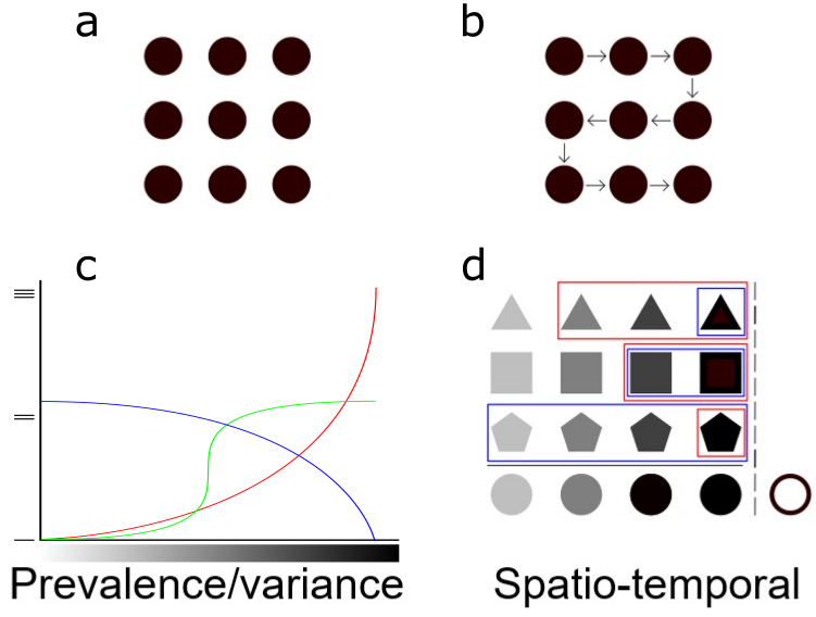
Figure 1 Modeling approaches for a river system: prevalence/variance vs spatio-temporal. a-b) Sites are treated as independent for the prevalence/variance approach; dependence between sites is taken into account for the spatio-temporal analysis. c) The prevalence/variance method looks at variations in microbial community composition along gradients. The various curves represent different taxa shifting in abundance along a gradient. d) The spatio-temporal method uses bacterial taxa abundances in various transformations taking into account the spatio-temporal dependency between sites in order to predict downstream ecological outcomes. Pictogram transparency represents distance and time gradients across sampling sites.
How should we select which bacterial taxa to include in our models? What happens if one combination of species works as well as another and how often does this happen? Is there a gradient of usefulness across bacterial taxa in terms of model predictive power? These questions all point to information content. There is a certain amount of information required for predictive models to yield accurate predictions. Our objective thus turned to extracting this informational keystone from data. To achieve this, we chose to use model resampling. The idea is to build models one bacterial taxa at a time, adding them to the model if they yield improved accuracy. This screening process was repeated with randomly ordered bacterial taxa. The randomization allowed for each taxa to have a chance to be added to a model if they contain useful information. Once this screening process had been run a great many times, we summed the number of times each taxa showed up in a model and which taxa never showed up together. These two elements gave an estimate of how much information each taxa contains as well as which taxa contain redundant information. In this latter case, taxa are not added to the same models during the iterative process. In the end, we visualized these information contents in the form of co-occurrence and co-exclusion networks.
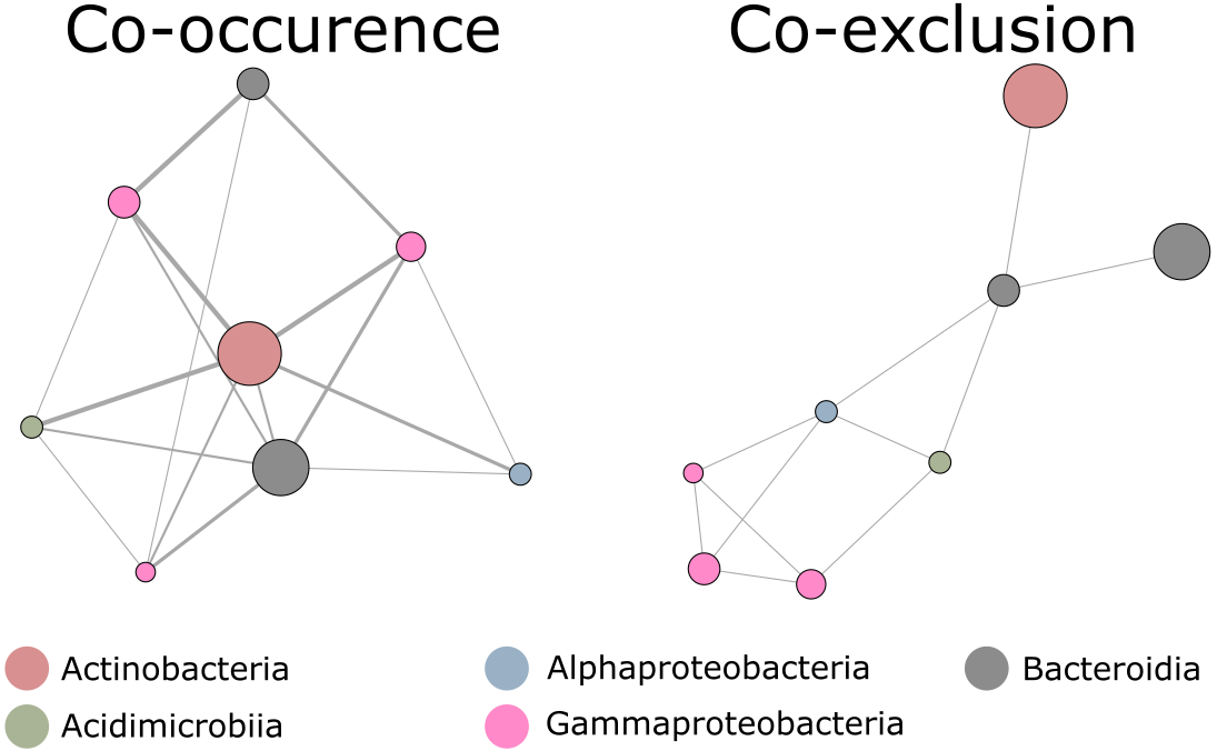
Figure 2 Network analysis results for the most frequent taxa returned by the spatio-temporal approach yielding perfectly accurate ecological status classification. Nodes represent individual taxa. Colors represent the respective bacterial classes to which taxa belong. Co-occurrence network; node diameter represents the number of occurrences of each taxon in the best models, while the thickness of the connecting lines represents the number of co-occurrences of taxa pairs. Co-exclusion network; links represent taxa that never occurred together in the same model. Adapted from Figure 4 in the article.
What would an ideal bioindicator look like? A good bacterial predictor ought to be present along the widest possible stretch of an environmental gradient and display sufficient variation to link its abundance to specific ecological outcomes. The importance of a broad distribution together with wide variations in abundance rests with the objective of needing as few as possible bioindicators to yield a complete picture. Specialist taxa could be very informative about relevant processes but the possibility of competitive exclusion means more than one may have to be included in a model to account for a given ecological process. In summary, good bioindicators would occupy a wide multidimensional niche space that does not overlap with other taxa.
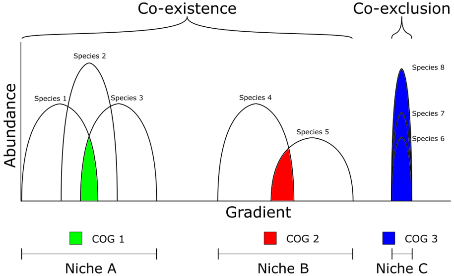
Figure 3 Hypothetical functional signals and niche dynamics across an environmental gradient. Functional diversity is represented as Clusters of Orthologous Genes (COG). Bell-shaped curves represent niche space for each species along a given environmental gradient.
How does one distinguish real patterns from noise? Meaningful signals in microbial ecology datasets are often difficult to capture. We can easily detect broadly linear relationships with matrix inversion-based methods, but non-linear patterns are a lot harder to pick up and may require different tools. Complex relationships are more susceptible to detection when using machine learning algorithms such as neural networks or tree-based methods. We opted for one of the latter, XGBoost, as it performs well on high dimensional data with relatively low observation counts.
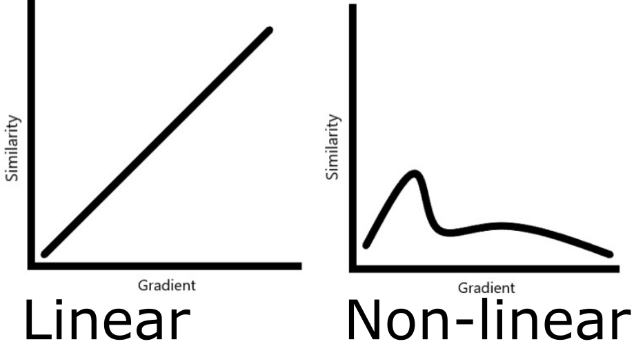
Figure 4 Hypothetical beta diversity patterns across environmental gradients. The linear one is easily detectable while the other isn’t. The latter is common in natural systems.
To which degree can one characterize processes from abundance tables and environmental metadata? Microbial ecology data is practically always noisy, complex and incomplete. It is challenging in these conditions to find meaningful patterns that can be translated into a mechanistic understanding, particularly without experimental data to provide a starting point in the search for causality. A common problem arises from observational studies and the urge to assign cause and effect. While we can never rigorously ascribe causality without experimentation, it is certainly possible to engage in well-supported hypothesis generation by proving the relevance of identified relationships through predictive modeling. If one can consistently generate accurate predictions for input data a model was neither trained nor calibrated on, the model is solid and contains kernels of truth. In other words, the proof is in the pudding. Once satisfactory predictions are achieved, one can examine the models and look into which variables are relevant and how they interact, as is relatively straightforward with tree-based methods. This information can then be used to formulate hypotheses that can be verified experimentally.
Follow the Topic
-
Communications Biology

An open access journal from Nature Portfolio publishing high-quality research, reviews and commentary in all areas of the biological sciences, representing significant advances and bringing new biological insight to a specialized area of research.
Related Collections
With Collections, you can get published faster and increase your visibility.
From RNA Detection to Molecular Mechanisms
Publishing Model: Open Access
Deadline: May 05, 2026
Signalling Pathways of Innate Immunity
Publishing Model: Hybrid
Deadline: May 31, 2026



Please sign in or register for FREE
If you are a registered user on Research Communities by Springer Nature, please sign in