A stopwatch for light

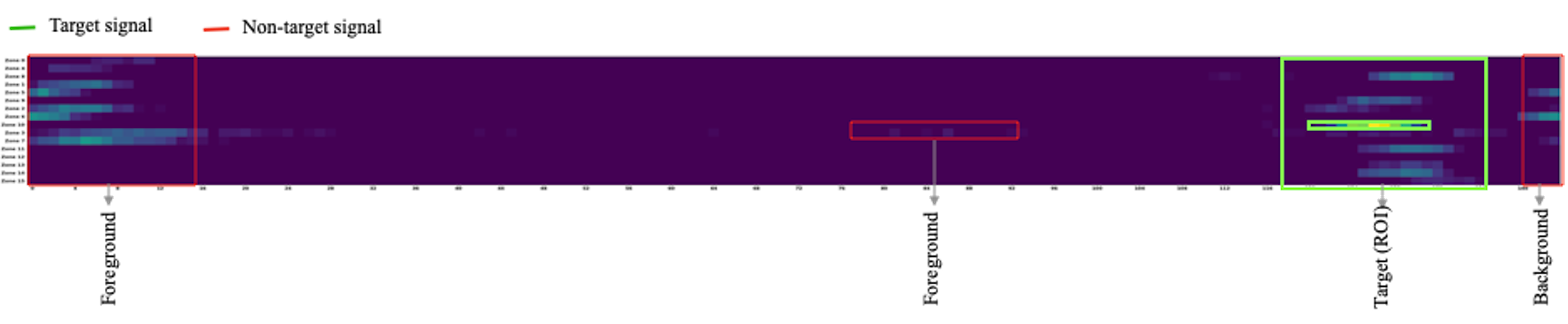
Time-of-flight (ToF) sensors estimate distance by measuring the delay between emitted light and detected return. For a simple round-trip measurement, d = cΔt/2. The factor of two accounts for the outward and return journeys. Real devices use different illumination and readout schemes, but the central idea is the same: timing gives information about the path travelled by light. A direct ToF system may emit short pulses and measure arrival times of returning photons. A sensor can accumulate these measurements into a histogram, where peaks and tails represent the temporal distribution of detected events. This distribution is influenced by the target, optical path, illumination and instrument response .

What SPADs contribute

A single-photon avalanche diode (SPAD) is operated so that the detection of a photon can trigger a measurable electrical pulse. With appropriate timing electronics, arrays of SPADs can register photon arrivals with fine temporal resolution. This makes them useful when the returning signal is weak or when the time structure of light carries information beyond integrated intensity. SPAD systems are not free of limitations. Dark counts create events without a detected scene photon; dead time limits how quickly a detector can register successive events; afterpulsing and timing jitter can distort measurements; and bright background light can overwhelm the signal . Histogram formation, time-to-digital conversion, data movement and power consumption are also important engineering constraints. Sensor architecture determines which information is available to an algorithm and at what cost.

In a simplified linear model the measured histogram h(t) can be written as

h(t) = (p * m * r)(t) + n(t)

where *p* is the emitted pulse shape, *m* the material (or scene) impulse response, *r* the instrument response function, * denotes convolution, and *n* collects dark counts, ambient light and other noise. Material-aware algorithms seek structure in *m* that survives the convolution and noise.

Could arrival-time distributions distinguish materials?

A material changes light through reflection, absorption, transmission and scattering. In a simplified setting, a smooth opaque surface may return a relatively concentrated response, whereas a translucent or strongly scattering material may produce a broader distribution of photon arrival times. This intuition motivates research into using transient or time-resolved measurements for material classification. However, arrival-time distributions are not intrinsic fingerprints in isolation. They depend on distance, surface orientation, illumination wavelength, angle of incidence, surrounding geometry, detector response and ambient light. A dark surface may yield few detected photons; a reflective surface can cause saturation or multipath effects; and two different materials may have similar measured responses under a particular setup. Reliable classification therefore requires experiments that vary these conditions and test whether a model has learned material-related cues rather than shortcuts tied to the laboratory or sensor.

Fusion: let each sensor do what it measures best

A practical architecture can combine an RGB camera with a time-resolved sensor. The RGB stream offers strong spatial detail and familiar appearance cues. The temporal stream may contribute distance and information about the way light returns. One approach is to detect an object in the RGB image, align the corresponding region with time-resolved data, and then estimate a material class from temporal features. Another is to fuse features earlier in a neural network. Neither strategy is automatically superior. Early fusion can learn complex interactions but may be sensitive to calibration and missing data. Late fusion is easier to interpret and can allow one stream to remain useful when the other is unreliable, but it may miss fine-grained cross-modal relationships. The right choice depends on the task, sensor arrangement, latency budget and failure costs. A system should also be allowed to abstain when evidence is weak rather than always returning a confident class.

Cross-feature sourcing formalises this division: spatial features (layout, category) are taken from laterally resolved intensity; material and range are taken from co-registered dToF transients . Dual-module pipelines built on that principle have reported combined spatial-material scores of roughly 94.5–98.5% on controlled categories and material-module validation near 99% at millisecond-class CPU inference, with explicit tests against LED-screen and print spoofing. Those results illustrate what is possible under a documented protocol; they do not yet generalise to unconstrained multi-object or outdoor scenes.

Evaluation should challenge the model

A credible material-recognition study should compare RGB-only, temporal-only and fused baselines using the same data partitions and evaluation protocol. It should report per-class performance, confusion matrices, uncertainty and performance under changes in illumination, distance, viewpoint and surface condition. Splitting data randomly at the frame level can overestimate generalisation if adjacent frames or repeated captures of the same object occur in both training and test sets. Splits by object, session or environment provide a more demanding test. Researchers should also examine photon efficiency: how does performance change when fewer photons are available or acquisition time is shortened? This matters for moving scenes and energy-constrained devices. Other useful measurements include latency, memory, energy consumption, sensor cost and calibration stability. An accuracy gain is most compelling when it persists outside the original acquisition conditions and justifies additional hardware and computation.

Where the research could lead

Time-resolved sensing could support industrial inspection, robotic manipulation and other applications where appearance alone is ambiguous. But the strongest case will be made through clearly bounded claims: which material categories can be distinguished, under what optical conditions, with what uncertainty and at what cost? Open datasets that include raw timing histograms, sensor metadata, calibration procedures and environmental variation would make results easier to reproduce. Benchmarking should include difficult negatives and unknown materials, not only classes seen during training. Physics-informed features may help reduce dependence on large labelled datasets, while learned models may capture patterns that simple summary statistics miss. Comparing both approaches could reveal when data-driven complexity is justified.

ToF is often introduced as a way to measure distance. Its broader promise is to turn the time structure of detected light into useful evidence about the scene. Whether that promise translates into dependable material-aware vision beyond spatial appearance depends on careful sensor design, realistic evaluation and transparent reporting of limitations.

References

[1] Piron, F. et al. "A review of single-photon avalanche diode Time-of-Flight imaging sensor arrays." IEEE Sensors Journal 21(11), 12654–12666 (2021).
[2] Bruschini, C. et al. "Single-photon avalanche diode imagers in biophotonics: review and outlook." Light: Science & Applications 8, 87 (2019).
[3] Minka, D. A. "Beyond Appearance: Intelligent Spatiotemporal Vision for Material-Aware Object Detection." Research Square preprint (2026).