Initiation

It was a long story…

From the very beginning, this work was started at a discussion meeting with Profs. Haoyu Li and Liangyi Chen. At that time, we were developing deep-learning super-resolution microscopy. Although the generated results were rather beautiful, we were still unsatisfied with the current assessment solutions, such as using PSNR (peak signal-to-noise ratio) or SSIM (structural similarity) calculated against ground-truth. First, these metrics are sensitive to background and intensity fluctuations, and is difficult to truly reflect the supe-resolution quality. Second and most importantly, when we put the deep-learning engine into real usage, we usually don't have the access to the corresponding ground-truth.

This is also relevant to the classical super-resolution techniques. The noise and distortions in raw images caused by the photophysics of fluorophores, the chemical environment of the sample, and the optical setup conditions, may influence the qualities of the final super-resolution images. We also expect the in situ evaluation for every specific experiment.

Thus, to evaluate the super-resolution quality in general, we intend to create a model-independent or model-agnostic solution, i.e., rFRC (rolling Fourier ring correlation). The very first attempt was established by the Henriques lab, using the corresponding diffraction-limit image as reference. However, in addition to the need for wide-field reference, the RSM (resolution-scaled error map) as well as the FRC (Fourier ring correlation) map are still too coarse to describe the super-resolution scale spatial separation of the quality variation.

The upscaled resolvability of super-resolution imaging requires a more elaborate evaluation.

Model bias and data uncertainty

Before introducing our solution in detail, it is important to clarify the conceptual classification for the reconstruction errors. Systematically, we summarized that the reconstruction qualities of the corresponding super-resolution modalities are influenced by two types of degradation, i.e., the model bias and the data uncertainty. The model-bias-induced errors (model error) (right, Fig. 1b) are primarily caused by the difference between the artificially created estimation model and its physical, real-world counterpart, which can be detected and minimized by carefully calibrating the optical microscopy system and measuring its characteristics. On the other hand, the data uncertainties (left, Fig. 1b) are mostly introduced by joint effects of the noise condition and sampling capability of the hardware equipment, such as the sensors and cameras in microscopy systems. In other words, the reconstructions from the inevitably deviated observations (left panel of Fig. 1a) may also break away from the real-world objects in the target SR domain (right panel of Fig. 1a). Therefore, the data uncertainties are generally inevitable, hard to be suppressed by system calibrations, and free from the model, which may be more critical in quantitative biological-image analysis.

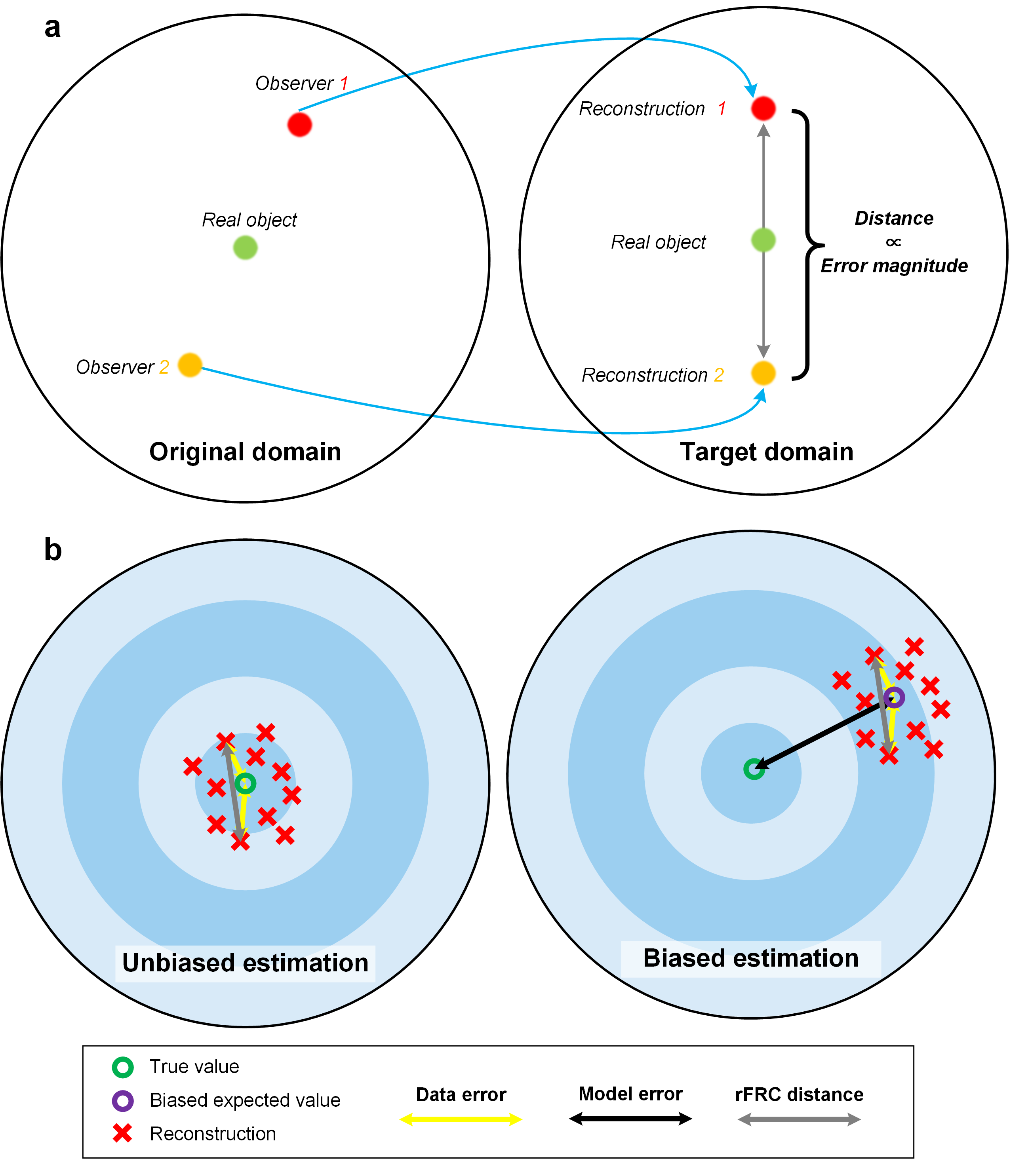
Fig. 1 | rFRC distance. (a) The basic concept of rFRC evaluation. The observer in the original domain indicates the captured raw images, and the reconstruction in the target domain represents the reconstructed SR images. (b) The data uncertainty, the model error, and the rFRC distance. The unbiased estimation indicates that the reconstruction model accurately describes the corresponding real-world model. Then the expected value of reconstructions will be identical to the actual value (green circle). The biased estimation represents that the reconstruction model is different from the real-world one. The expected value (purple circle) of reconstructions will deviate from the actual value (black arrow, model error).

Our solution

Heuristically, if two measurements are conducted on the same sample and considering the proper reconstruction model used, the distance between the two reconstructions may correlate to the data uncertainty (unbiased estimation, Fig. 1b). In this sense, we can use this distance (Reconstruction 1 versus Reconstruction 2) to approximate the magnitude of the reconstructed error. Heuristically, we can capture statistically independent images of the object by imaging the identical object with the same configurations. The data uncertainties can be highlighted by the difference between these individual reconstructions (Fig. 1a).

In this sense, the conventional pixel-wise spatial evaluation methods, such as spatial subtraction or standard deviation of the individually reconstructed results may quantify the distance between the recorded images. However, by measuring the 'absolute differences', the subtraction between this image pair is susceptible to the intensity fluctuation and subpixel structural motions, producing false negatives in distance maps that overshadow genuine errors. To minimize the false negatives, we repurposed the FRC to quantify the distance between two individual SR reconstructions in the Fourier domain. By calculating the 'relative error' or 'saliency-based error', the FRC is insensitive to intensity fluctuations or structure movements, thus more robust (Fig. 2). To provide local distance measurements, we transformed the conventional FRC framework into a rolling FRC (rFRC) map, which directly evaluated spatial information at the SR scale.

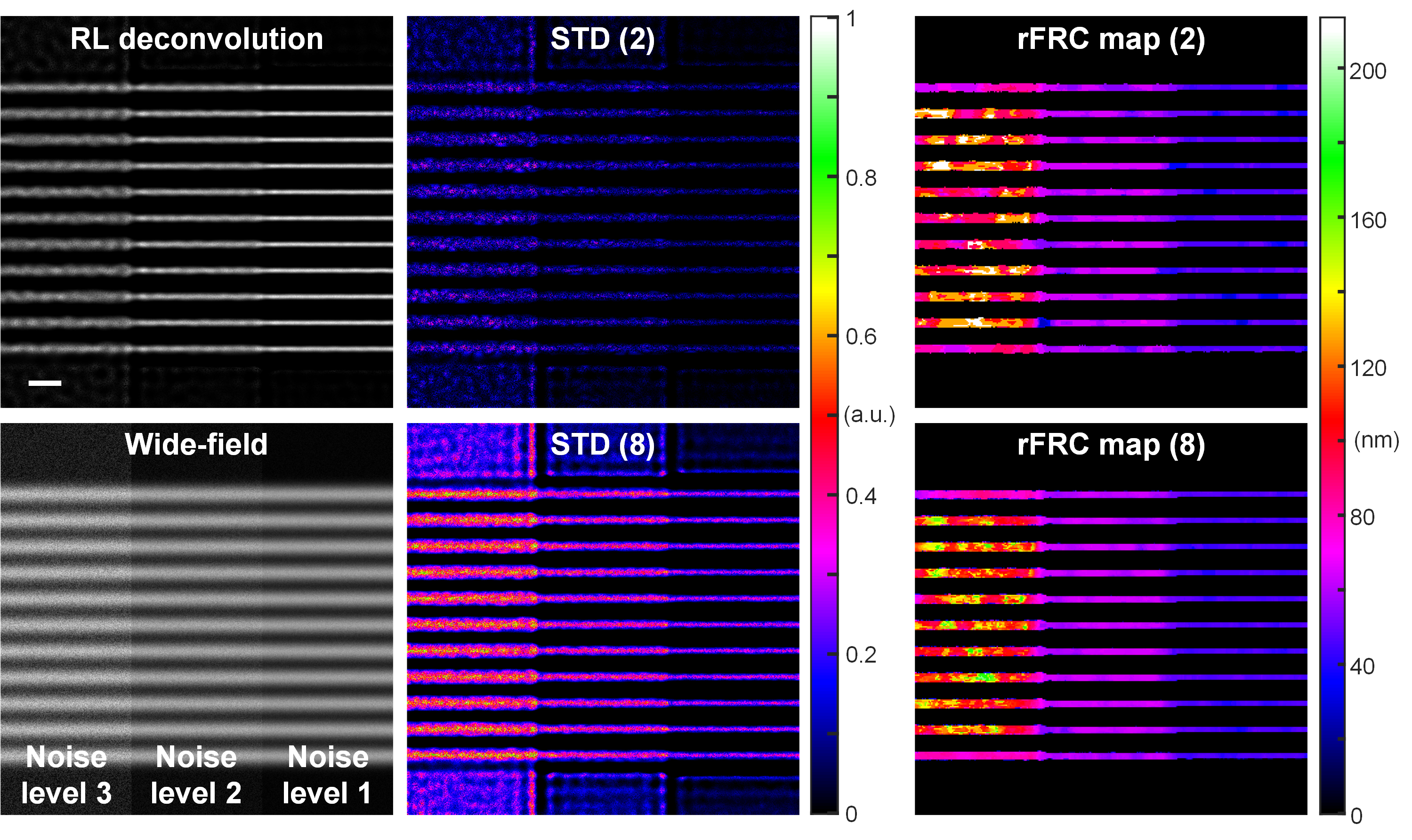
Fig. 2 | Evaluations in spatial domain versus Fourier domain. A series of filaments were convoluted with a wide-field PSF (numerical aperture as 1.4). We gradually decreased the noise level from left to right in three levels (left bottom). Left top: RL deconvolution result. Middle: STD (standard deviation) results of 2 (top) and 8 (bottom) RL deconvolved images. Middle: rFRC map of 2 (top) and 8 (bottom) RL deconvolved images. The 8 images were splitted into 4 batches for rFRC mapping, and the 4 resulting rFRC maps were averaged to create the final rFRC map (8). Scale bar: 500 nm.

Evaluating the union set of classical and deep-learning microscopies

In the very first version (see this bioRxiv preprint), Prof. Liangyi was keen to include the evaluation of deep-learning microscopy as it was the start point of this work. I and Prof. Haoyu were also very excited about the successful assessments of different types of deep-learning microscopy techniques as shown in the preprint. However, after a long and painful two-round appeal in Nature Methods, we realized that this ambition may go too far, at least for the current stage. Thus, although being reluctant, we shrank our topic to only classical super-resolution microscopy evaluation and submitted it to another journal, Light: Science & Applications. Predictably, at this time, our story was more easily accepted by the reviewers.

rFRC and PANEL

We also offer two optional colormaps that may be more suitable for human intuition (than Jet) to display the uncertainties (shifted Jet, sJet; and black Jet, bJet) (Fig. 3a).

Fig. 3 | Color maps for map display and Otsu threshold for PANEL pinpointing. (a) The representative color-coded images and color indexes of jet (left), black jet (middle), and shifted jet (right) color maps. (b) Otsu threshold for PANEL highlighting. Left: The rFRC map of the SRRF dataset, displayed in the sJet color map. Middle and right: The Full rFRC map (middle) and the rFRC map after the Otsu threshold (right), regions with low reliability in the SRRF reconstruction are pointed by green.

By involving the rolling operation, we have addressed a major limitation of the previous FRC map, which is challenging to correlate the block-wise map to the SR image content. Here, in Fig. 4, are the systematic comparisons of our rFRC map against the FRC map.

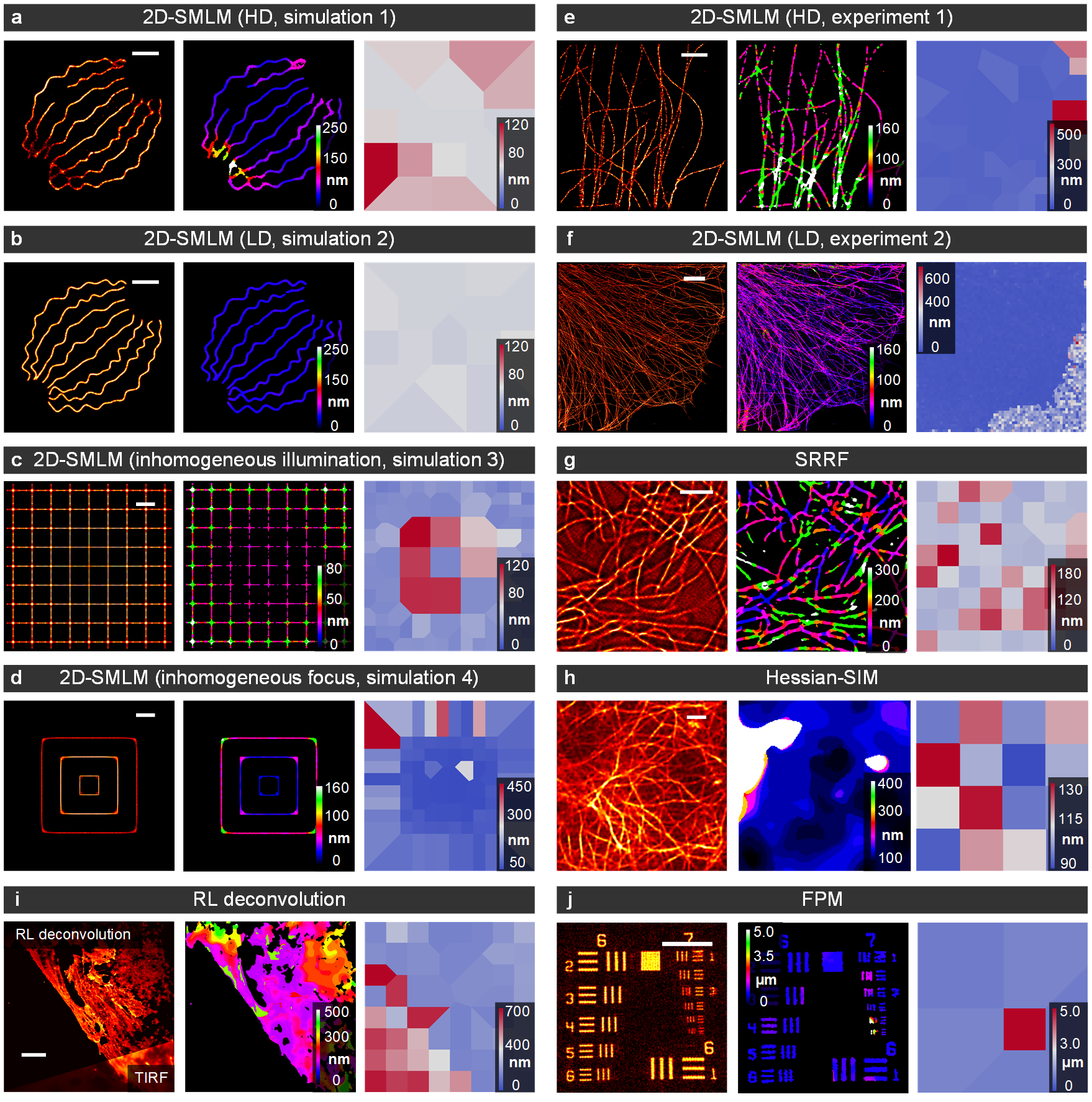
Fig. 4 | rFRC maps versus FRC maps from different modalities. From left to right: Imaging data, rFRC map, and FRC map. (a, b) 2D-SMLM simulations with high-density ('HD', a) and low-density ('LD', b) emitting fluorophores in each frame (c.f., Fig. 2a). (c) 2D-SMLM simulation with inhomogeneous illumination (c.f., Fig. 2b). (d) 2D-SMLM simulation with inhomogeneous focus (c.f., Fig. 2c). (e, f) 2D-SMLM experiments with high-density ('HD', e) (c.f., Fig. S7a) and low-density ('LD', f) (c.f., Fig. 3f) emitting fluorophores in each frame. (g) SRRF experiment (c.f., Fig. S7c). (h) Hessian-SIM experiment (c.f., Fig. 6a). (i) RL deconvolution experiment (c.f., Fig. 6d). (j) FPM simulation (c.f., Fig. 6h). The FRC map is based on the 1/7 fixed threshold, which may generate unstable calculations. Hence, an inverse distance weight function is involved in interpolating values in all FOVs, while the FRC resolution might not be obtained. This strategy and the calculation on background areas may generate strong false negatives in the resulting FRC map. Scale bars: (a, b) 500 nm; (c, d, h) 1 μm; (e, g) 2 μm; (f, i) 5 μm. (j) 50 μm. Indexes in this caption are corresponding to the figures in our article.

Importantly, the rFRC may not identify the regions that were always incorrectly restored during different reconstructions due to the model bias. For example, if the two reconstructed images lost an identical component, the rFRC may indicate a false positive in the corresponding region. To moderate this issue, we combined a modified RSM with our rFRC to constitute the PANEL, for pinpointing such regions with low reliability. As small intensity fluctuations can lead to potential false negatives, we truncated the RSM with a hard threshold (0.5), only including prominent artifacts such as misrepresentations or the disappearance of structures. To filter the regions with high quality (high FRC resolution), we adopted the Otsu-based segmentation to highlight regions giving a higher probability of the error existence (Fig. 3b). We then merged the filtered rFRC map (green channel) and RSM (red channel) to create the composite PANEL map. Note that our PANEL cannot fully pinpoint the unreliable regions induced by the model bias at present, which would require more extensive characterization and correction routines based on the underlying theory of the corresponding models.

Here is also a comparison between PANEL and SQUIRREL:

Open-sourced resources

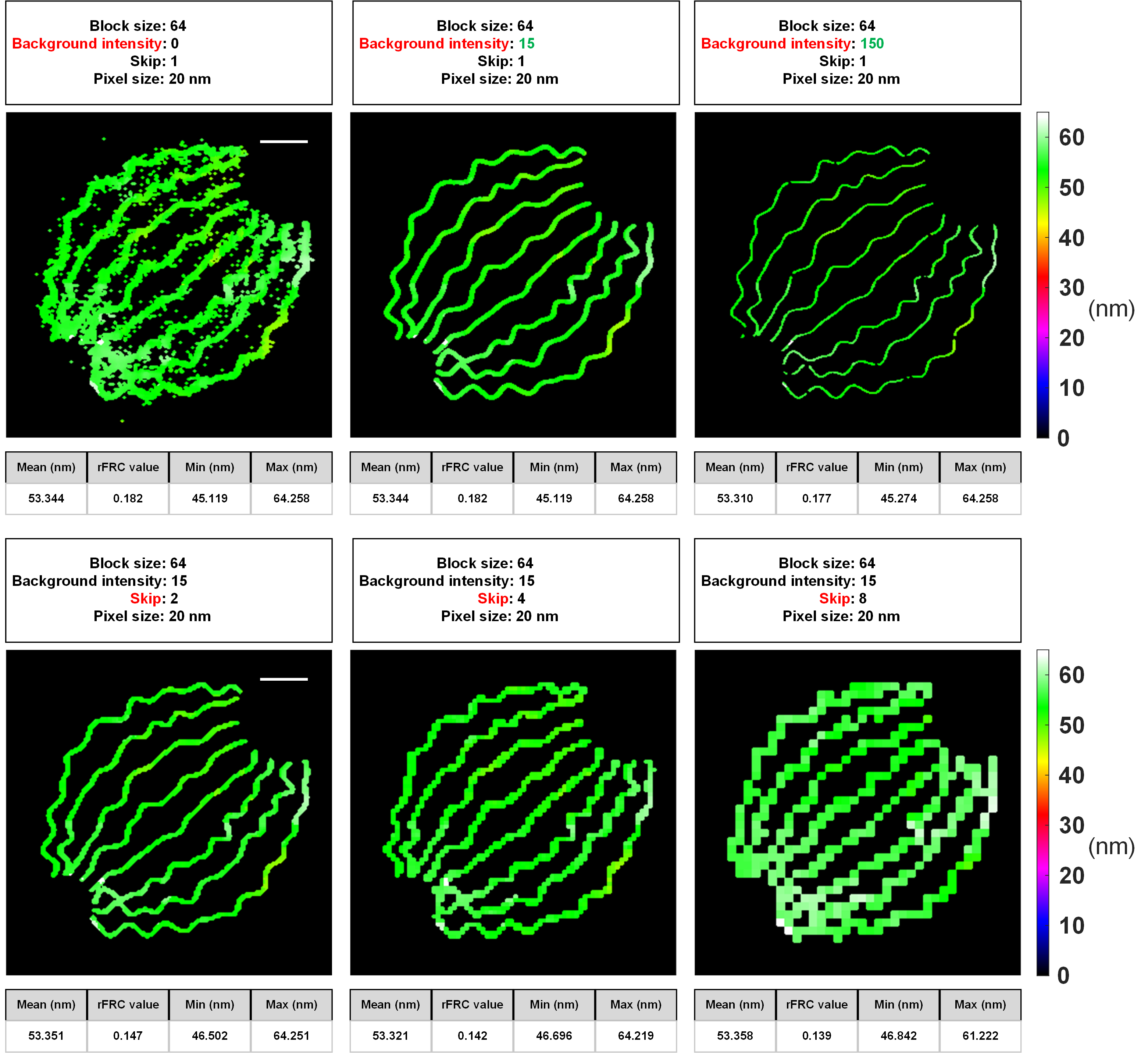
We have provided the MATLAB code, Python code, and FIJI/ImageJ plugin for rFRC calculation. Currently, the full version of PANEL can only be found in the MATLAB version. The FIJI/ImageJ plugin and Python version only support rFRC calculation and PANEL pinpointing without RSM.

As we have shown in the GitHub wiki, our PANELJ plugin can be executed smoothly for evaluating local resolutions at different scales:

At the end

Again, the upscaled resolvability of super-resolution imaging requires a more elaborate evaluation. In this work, we developed rFRC for detecting data uncertainty of super-resolution images at the corresponding super-resolution scale without any referencing. The combination of rFRC map and filtered RSM, PANEL, can reflect part of model-bias-induced errors, and this solution is focusing on the classical super-resolution microscopy.

Delightfully, we will soon release a new version focusing on the evaluation of deep-learning microscopy, regarding the full data uncertainty and model uncertainty assessment.